5 Ways to Format Cells in Google Sheets
Updated on

Google Sheets is a powerful spreadsheet tool that allows users to organize, analyze, and share data. With its various cell formatting options, users can make their data more visually appealing and easier to understand. Here are 5 ways to format cells in Google Sheets:
Need additional help? Want to try something more advanced than Google Sheets?
We are offering an Open Source Data Analysis Tool that is ready Out-of-the-Box.
Explore Data with RATH (opens in a new tab) Now.
1. Use Basic Cell Formatting Options
Google Sheets offers several basic cell formatting options, such as font formatting, number formatting, alignment, and borders.
-
Font formatting allows users to change the font size, style, and color of the text.
-
Number formatting is used to format numerical data, including dates, currency, and percentages.
-
Alignment allows users to change the position of the text within a cell, such as left, center, or right.
-
Borders are used to create a border around a cell or range of cells.

2. Try Advanced Cell Formatting Options
Google Sheets also offers advanced cell formatting options, such as conditional formatting, data bars, and color scales.
-
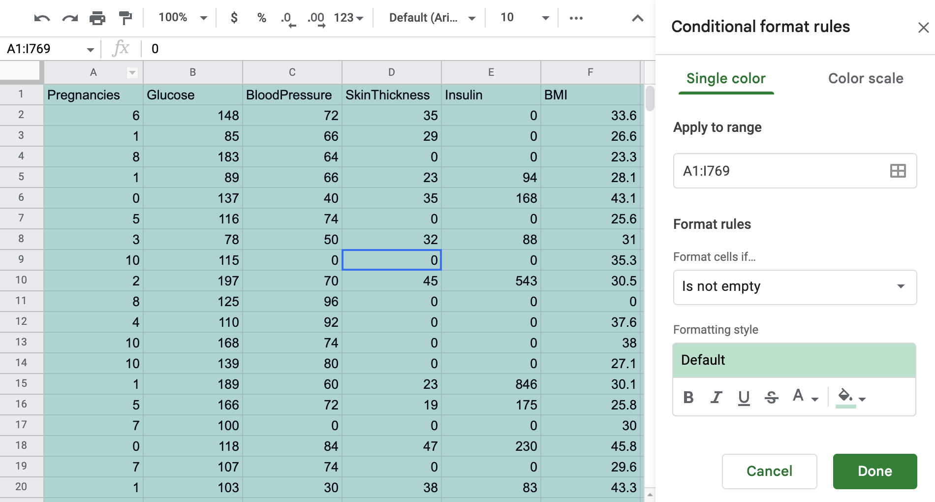
Conditional formatting allows users to format cells based on specific conditions, such as if a cell contains a certain value or if it's based on another cell. This feature is especially useful for highlighting duplicate values or values that meet specific criteria.
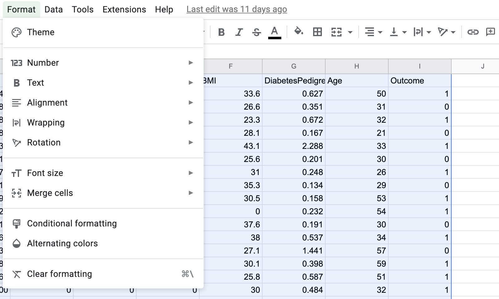
To use Google Sheets conditional formatting based on another cell, users need to select the range of cells and then choose the Format -> Conditional Formatting option in the menu. They can then enter the formula based on the conditions they want to use.

-
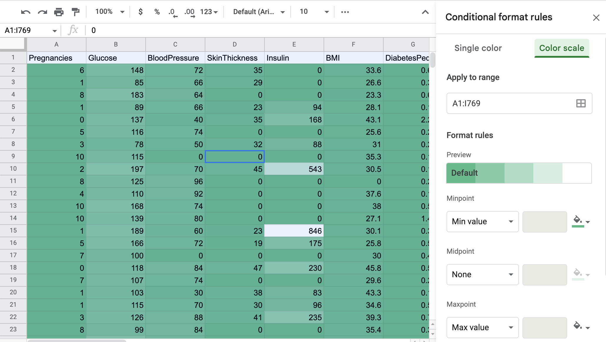
Color scales are used to visualize data more graphically. Color scales allow users to color-code cells based on their values, making it easier to identify trends and patterns in data.

3. Use Custom Cell Formatting Options
In addition to the standard formatting options, Google Sheets also offers custom cell formatting options.
-
Format a cell as text: This can prevent Google Sheets from automatically formatting the data. This is useful for data that includes numbers with leading zeros or data that should be treated as text.
To format a cell as text in Google Sheets, simply select the cell(s), right-click and choose Format cells. In the "Number" tab, select "Plain text" and click "Apply". The cell(s) will now be formatted as text.
-
Use conditional formatting based on another sheet: This is helpful when comparing data across multiple sheets or when referencing data that's not in the current sheet. To use Google Sheets conditional formatting based on another sheet, users need to enter the sheet name and cell range in the formula:
=IF(Sheet1!A1>10,TRUE,FALSE).
4. Remove Duplicates Using Conditional Formatting
Google Sheets also offers a quick way to highlitht duplicates using conditional formatting.
To use Google Sheets conditional formatting duplicates, users need to select the range of cells, go to the "Format" menu, and choose "Conditional formatting". They can then select the "Duplicate values" option, and Google Sheets will highlight the duplicate values.
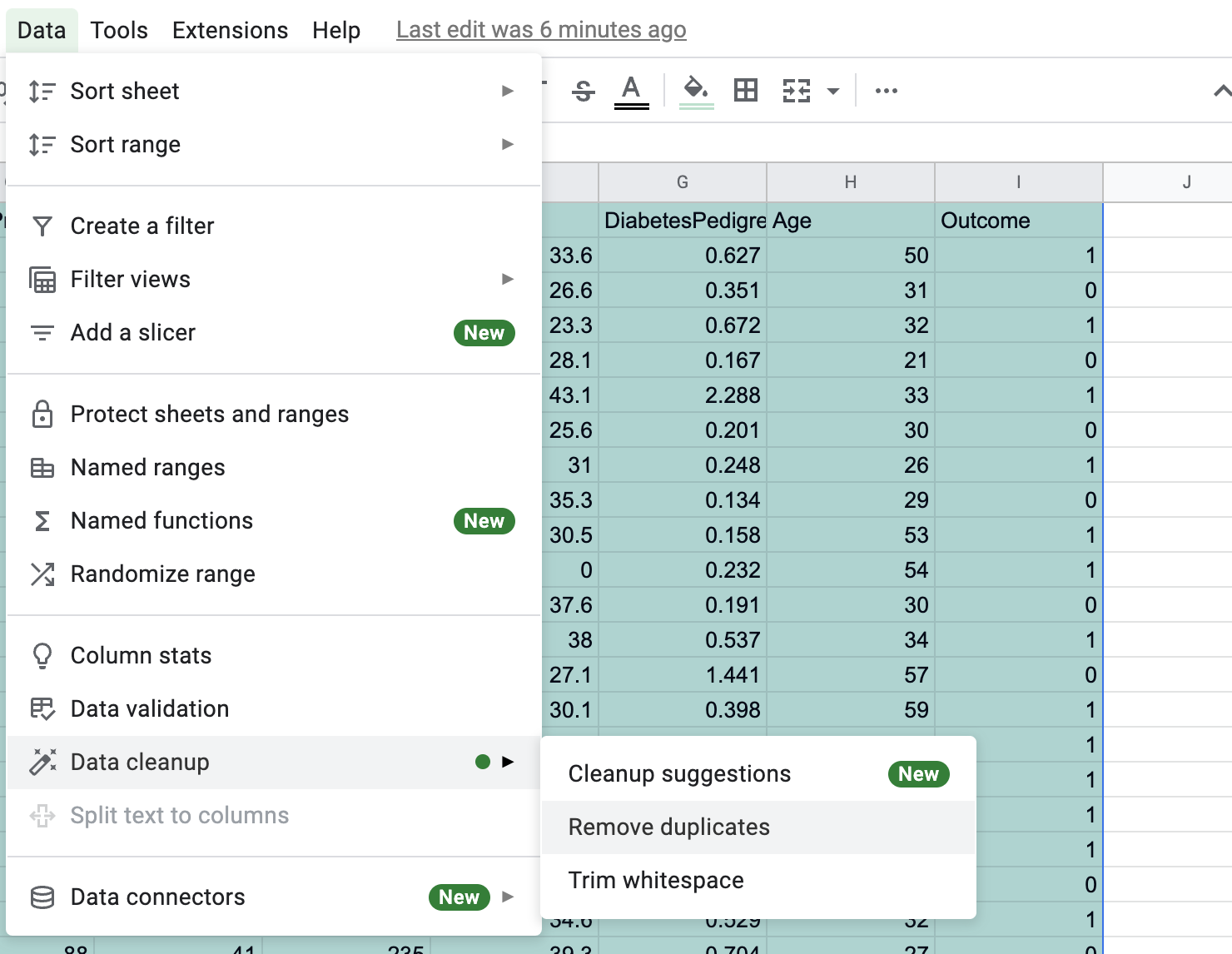
While conditional formatting can highlight duplicates in Google Sheets, it does not actually remove them. To remove duplicates, click on the Menu bar and choose Data -> Data cleanup -> Remove duplicates.

5. Highlight Cells That Meet Specific Criteria
Another useful feature of Google Sheets conditional formatting is the ability to highlight cells that meet specific criteria. For example, users can highlight cells that contain a certain word or phrase, or cells that are above or below a certain value.
To use this feature, users need to select the range of cells, go to the "Format" menu, and choose "Conditional formatting." They can then select the "Format rules" option and enter the formula based on the criteria they want to use.
Conclusion
In conclusion, Google Sheets offers a variety of cell formatting options to help users make their data more visually appealing and easier to understand. By using basic formatting options such as font, alignment, and borders, as well as advanced options such as conditional formatting, data bars, and color scales, users can create professional-looking spreadsheets.
