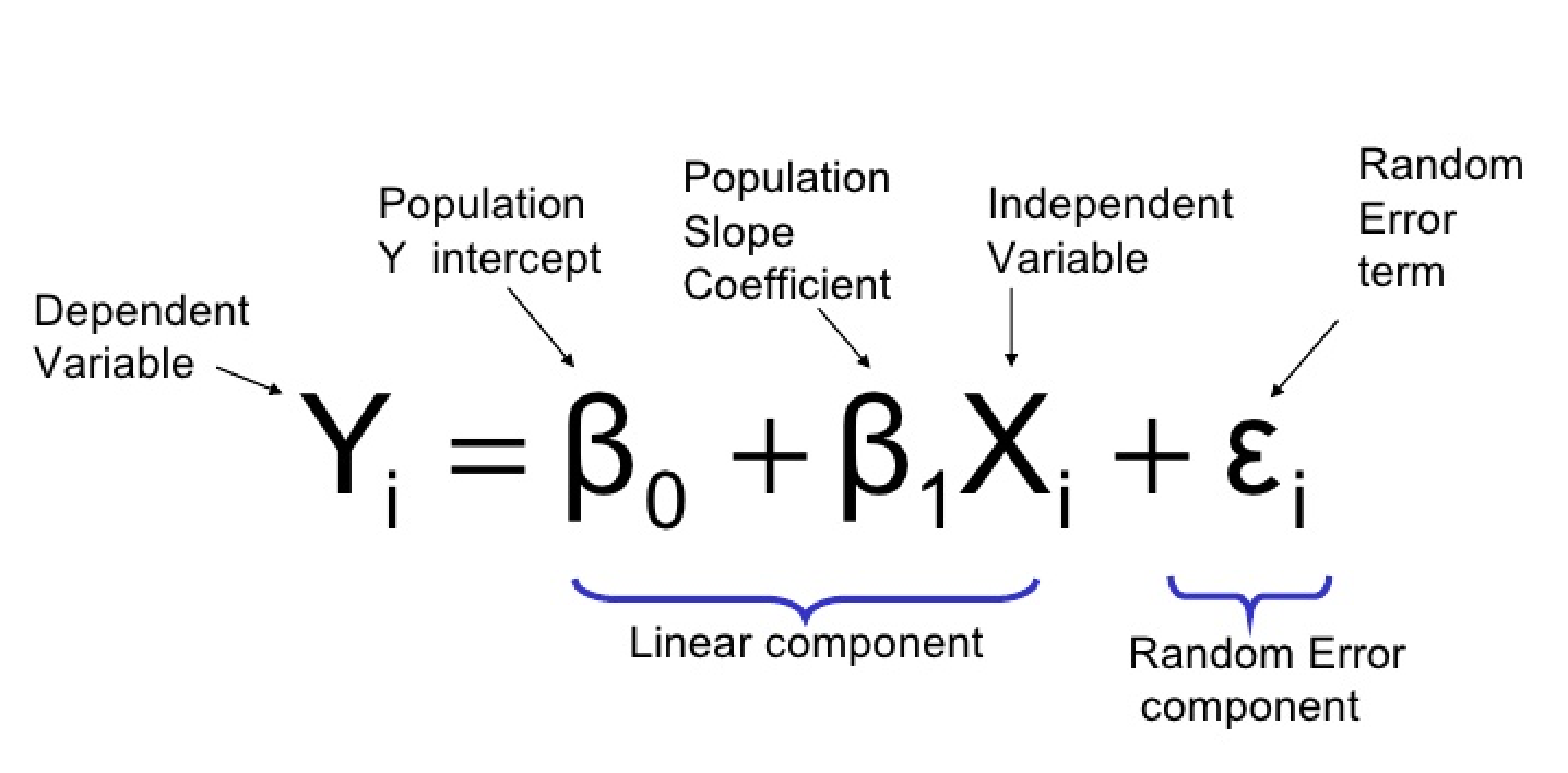
Logistic Regression Equation in R: Understanding the Formula with Examples

Name: Rajiv Chandra

Updated on 4/20/2022

Logistic regression is one of the most popular statistical techniques used in machine learning for binary classification problems. It uses a logistic function to model the relationship between a dependent variable and one or more independent variables. The goal of logistic regression is to find the best relationship between the input features and the output variable. In this article, we will discuss the logistic regression equation with examples in R.

Want to quickly create Data Visualization from Python Pandas Dataframe with No code?

PyGWalker is a Python library for Exploratory Data Analysis with Visualization. PyGWalker (opens in a new tab) can simplify your Jupyter Notebook data analysis and data visualization workflow, by turning your pandas dataframe (and polars dataframe) into a tableau-alternative User Interface for visual exploration.

(opens in a new tab)

Logistic Regression Equation

The logistic regression equation can be defined as follows:

Logistic Regression

where:

Y: the dependent variable or response variable (binary)
X1, X2, …, Xp: independent variables or predictors
β0, β1, β2, …, βp: beta coefficients or model parameters

The logistic regression model estimates the values of beta coefficients. The beta coefficients represent the change in the log-odds of the dependent variable when the corresponding independent variable changes by one unit. The logistic function (also called the sigmoid function) then transforms the log-odds into probabilities between 0 and 1.

Applying Logistic Regression in R

In this section, we will use the glm() function in R to build and train a logistic regression model on a sample dataset. We will use the hr_analytics dataset from the RSample package.

Loading Data

First, we load the required package and dataset:

library(RSample)
data(hr_analytics)

The hr_analytics dataset contains information about employees of a certain company, including their age, gender, education level, department, and whether they left the company or not.

Preparing Data

We convert the target variable left_company into a binary variable:

hr_analytics$left_company <- ifelse(hr_analytics$left_company == "Yes", 1, 0)

Next, we split the dataset into training and test sets:

set.seed(123)
split <- initial_split(hr_analytics, prop = 0.7)
train <- training(split)
test <- testing(split)

Building the Model

We fit a logistic regression model using the glm() function:

logistic_model <- glm(left_company ~ ., data = train, family = "binomial")

In this example, we use all the available independent variables (age, gender, education, department) to predict the dependent variable (left_company). The family argument specifies the type of model we want to fit. Since we are dealing with a binary classification problem, we specify "binomial" as the family.

Evaluating the Model

To evaluate the performance of the model, we use the summary() function:

summary(logistic_model)

Output:

Call:
glm(formula = left_company ~ ., family = "binomial", data = train)

Deviance Residuals: 
   Min      1Q  Median      3Q     Max  
-2.389  -0.640  -0.378   0.665   2.866  

Coefficients:
                     Estimate Std. Error z value Pr(>|z|)    
(Intercept)         -0.721620   0.208390  -3.462 0.000534 ***
age                 -0.008328   0.004781  -1.742 0.081288 .  
genderMale           0.568869   0.086785   6.553 5.89e-11 ***
educationHigh School 0.603068   0.132046   4.567 4.99e-06 ***
educationMaster's   -0.175406   0.156069  -1.123 0.261918    
departmentHR         1.989789   0.171596  11.594  < 2e-16 ***
departmentIT         0.906366   0.141395   6.414 1.39e-10 ***
departmentSales      1.393794   0.177948   7.822 5.12e-15 ***
---
Signif. codes:  0 ‘***’ 0.001 ‘**’ 0.01 ‘*’ 0.05 ‘.’ 0.1 ‘ ’ 1

(Dispersion parameter for binomial family taken to be 1)

    Null deviance: 6589.7  on 4799  degrees of freedom
Residual deviance: 5878.5  on 4792  degrees of freedom
AIC: 5894.5

Number of Fisher Scoring iterations: 5

The output shows the coefficients of the model (beta coefficients), their standard errors, z-value, and p-value. We can interpret the coefficients as follows:

The coefficients with a significant p-value (p < 0.05) are statistically significant and have a significant impact on the outcome. In this case, age, gender, education, and department are significant predictors of whether an employee leaves the company or not.
The coefficients with a non-significant p-value (p > 0.05) are not statistically significant and have no significant impact on the outcome. In this case, education level (Master's) is not a significant predictor.

Making Predictions

To make predictions on new data, we use the predict() function:

predictions <- predict(logistic_model, newdata = test, type = "response")

The newdata argument specifies the new data on which we want to make predictions. The type argument specifies the type of output we want. Since we are dealing with binary classification, we specify "response" as the type.

Evaluating Predictions

Finally, we evaluate the predictions using the confusion matrix:

table(Predicted = ifelse(predictions > 0.5, 1, 0), Actual = test$left_company)

Output:

         Actual
Predicted    0    1
        0 1941  334
        1  206  419

The confusion matrix shows the number of true positives, false positives, true negatives, and false negatives. We can use these values to calculate performance metrics such as precision, recall, and F1 score.

Conclusion

In this article, we discussed the logistic regression equation and how it is used to model the relationship between independent variables and a dependent binary variable. We also demonstrated how to use the glm() function in R to build, train, and evaluate a logistic regression model on a sample dataset. Logistic regression is a powerful technique for binary classification problems and is widely used in machine learning.